Random variables, expectations, and events¶

Suppose we’re interested in a random variable \(\omega\sim \textrm{Normal}(0, 1)\), i.e., \(\omega\) is a standard normal random variable.

In cvxstoc, we can declare this random variable like so:

from cvxstoc import NormalRandomVariable, expectation
omega = NormalRandomVariable(0, 1)

Now, intuitively, we might expect that as we average over more and more samples of this random variable (i.e., we compute \(\omega\)‘s sample mean over larger and larger samples), the sample mean will converge to zero. Let’s try to confirm this intuition using cvxstoc.

In cvxstoc, we can compute the sample mean like so (repeating some of the previous code for clarity):

from cvxstoc import NormalRandomVariable, expectation
omega = NormalRandomVariable(0, 1)
sample_mean = expectation(omega, 100).value

Here, 100 specifies the number of samples to use when computing the sample mean — we could have specified any natural number instead. As might be expected, sample_mean stores the (scalar) sample mean.

Indeed, if we execute this code for various values of the number of samples to use, and plot the resulting sample_mean values, we get this (confirming our intuition):

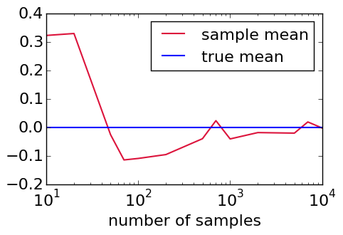
From this plot, we can see that the sample mean occasionally jumps above zero; so, one thing we might be further curious about is the probability that the sample mean (as a function of the number of samples) indeed lies above zero, i.e.,

In cvxstoc, we can compute this like so (by appealing to the Central Limit Theorem as well as repeating some of the previous code):

from cvxstoc import NormalRandomVariable, expectation, prob
omega = NormalRandomVariable(0, 1)                      # Not used, just here for reference
sample_mean = NormalRandomVariable(0, 1.0/100)          # This is the samp. dist. of the sample mean
bound = prob(0 <= sample_mean, 1000).value
print bound                                             # Get something close to 0.5, as expected

Here, prob takes in a (convex) inequality, draws samples of the random variable in question (1000 samples, in this case), evaluates the inequality on the basis of the samples, averages the results (just as in our experiments with the expected value from earlier), and (finally) returns a scalar; in other words

where \(1(\cdot)\) denotes the zero/one indicator function (one if its argument is true, zero otherwise) and \(\textrm{sample_mean}_i\) denotes the \(i\) th sample of the sample_mean random variable.

Yield-constrained cost minimization¶

Let’s combine all these ideas and code our first stochastic optimization problem using cvxstoc.

Suppose we run a factory that makes toys from \(n\) different kinds of raw materials. We would like to decide how much of each different kind of raw material to order, which we model as a vector \(x \in {\bf R}^n\), so that our ordering cost \(c^T x\), where \(c \in {\bf R}^n\) is a constant, is minimized, so long as we don’t exceed our factory’s ordering budget, i.e., \(x\) lies in some set of allowable values \(S\). Suppose further that our ordering process is error-prone: We may actually receive raw materials \(x + \omega\), where \(\omega \in {\bf R}^n\) is some random vector, even if we place an order for just \(x\). Thus, we can express our wish to not exceed our factory’s budget as

where \(\eta\) is a large probability, e.g., 0.95. Note that (2) is similar to (1); in general, (2) is referred to as a chance constraint (although in this context (2) is more often referred to as an \(\eta\)-yield constraint). Putting these considerations together leads us to the following optimization problem for choosing \(x\):

with variable \(x\).

We can directly express (3) using cvxstoc as follows (for simplicity, let’s take \(\omega \sim \textrm{Normal}(\mu, \Sigma)\), and \(S\) to be an ellipsoid):

from cvxstoc import NormalRandomVariable, prob
from cvxpy.expressions.variables import Variable
from cvxpy.atoms import *
from cvxpy import Minimize, Maximize, Problem
import numpy

# Create problem data.
n = 10
c = numpy.random.randn(n)
P, q, r = numpy.eye(n), numpy.random.randn(n), numpy.random.randn()
mu, Sigma = numpy.zeros(n), 0.1*numpy.eye(n)
omega = NormalRandomVariable(mu, Sigma)
m, eta = 100, 0.95

# Create and solve stochastic optimization problem.
x = Variable(n)
yield_constr = prob(quad_form(x+omega,P) + (x+omega).T*q + r >= 0, m) <= 1-eta
p = Problem(Minimize(x.T*c), [yield_constr])
p.solve()

(Much of the syntax for creating and solving the optimization problem follows from cvxpy.)

The news vendor problem¶

Let’s now consider a different problem (cf. page 16 in this book).

Suppose we sell newspapers. Each morning, we must decide how many newspapers \(x \in [0,b]\) to acquire, where \(b\) is our budget, e.g., the maximum number of newspapers we can store; later in the day, we will sell \(y \in {\bf R}_+\) of these newspapers at a (fixed) price of \(s \in {\bf R}_+\) dollars per newspaper, and return the rest (\(z \in {\bf R}_+\)) to our supplier at a (fixed) income of \(r \in {\bf R}_+\), in a proportion that is dictated by the amount of (uncertain) demand \(d \in {\bf R}_+ \sim \textrm{Categorical}\). We can model our decision-making process by the following optimization problem:

where

with variable \(x\).

Note that \(Q\) here is itself the optimal value of another convex optimization problem. The problem in (5)-(6) is referred to as a two-stage stochastic optimization problem: (5) is referred to as the first stage problem, while (6) is referred to as the second stage problem.

A cvxstoc implementation of (5)-(6) is as follows:

from cvxstoc import expectation, prob, CategoricalRandomVariable
from cvxpy import Minimize, Problem
from cvxpy.expressions.variables import Variable, NonNegative
from cvxpy.transforms import partial_optimize
import numpy

# Create problem data.
c, s, r, b = 10, 25, 5, 150
d_probs = [0.3, 0.6, 0.1]
d_vals = [55, 139, 141]
d = CategoricalRandomVariable(d_vals, d_probs)

# Create optimization variables.
x = NonNegative()
y, z = NonNegative(), NonNegative()

# Create second stage problem.
obj = -s*y - r*z
constrs = [y+z<=x, y<=d, z<=d]
p2 = Problem(Minimize(obj), constrs)
Q = partial_optimize(p2, [y, z], [x])

# Create and solve first stage problem.
p1 = Problem(Minimize(c*x + expectation(Q, num_samples=100)), [x<=b])
p1.solve()

Here, partial_optimize takes in a convex optimization Problem and a list of Variable s to optimize over — in this case, partial_optimize is given the (second stage) Problem named p2 and told to optimize (only) over the (second stage) variables y and z.